
Short description of article: Roberto’s article “An Introduction to Statistical Analysis and Modelling with Python is an extensive guide that addresses key aspects of statistical analysis and modeling using Python. The article begins with a discussion of graphical representations and plotting techniques. It then moves on to choosing the right functions for statistical modeling and details various parameter estimation methods. The author further explains the assessment of predictor accuracy and introduces various statistical tests, such as normality tests, to validate the models. Throughout the article, Roberto provides Python code examples, making it a practical resource for those looking to apply statistical methods in Python.
For a detailed read, the full article is available here. Also full article was copied and demonstrated below.
List of Contents:
- Introduction
- Graphical representations and plots
- Choosing the right function
- Parameter estimation
- Assessment of the goodness of a predictor
- Statistical tests
- Normality tests
Introduction
In statistical analysis, one of the possible analyses that can be conducted is to verify that the data fits a specific distribution, in other words, that the data “matches” a specific theoretical model.
This kind of analysis is called distribution fitting and consists of finding an interpolating mathematical function that represents the observed phenomenon.
An example could be when you have a series of observations 𝑥1,𝑥2,𝑥𝑛… and you want to verify if those observations come from a specific population described by a density function 𝑓(𝑥,θ), where θ is a vector of parameters to estimate based on the available data.
The main two purposes of statistical analysis are to describe and to investigate:
- To describe: estimate the moving average, impute missing data…
- To investigate: to search for a theoretical model that fits starting the observations we have.
This process can be break-down into four phases:
- Choosing the model that better fits the data
- Parameter estimation of the model
- Calculate the “similarity” between the chosen model and the theoretical model
- Apply a set of a statistical test to asses the goodness fo fit
Graphical representations and plots
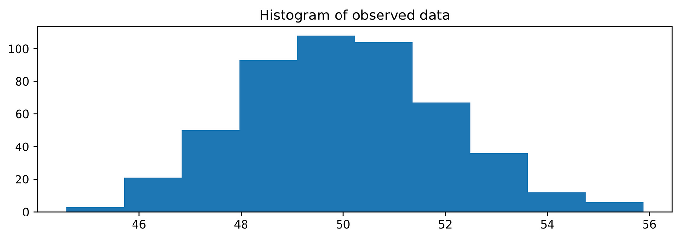
The first approach to explore data is graphical analysis. Analyzing the data graphically, with a histogram, can help a lot to assess the right model to choose.
Let’s draw a random sample of size 500, mean 50, and a standard deviation of 2 and plot a histogram:import numpy as npimport matplotlib.pyplot as pltx_norm = np.random.normal(50, 2, 500)plt.hist(x_norm)
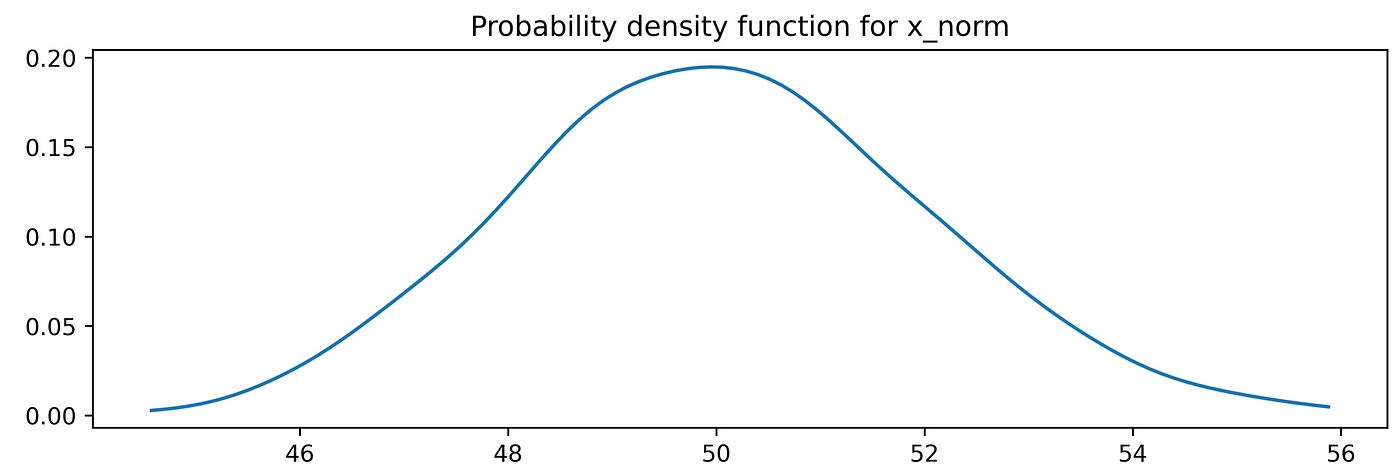
Another way to display our data is to estimate the probability density function:from scipy.stats.kde import gaussian_kdefrom numpy import linspace# estimate the probability density function (PDF)kde = gaussian_kde(x_norm)# return evenly spaced numbers over a specified intervaldist_space = linspace(min(x_norm), max(x_norm), 100)# plot the resultsplt.plot(dist_space, kde(dist_space))
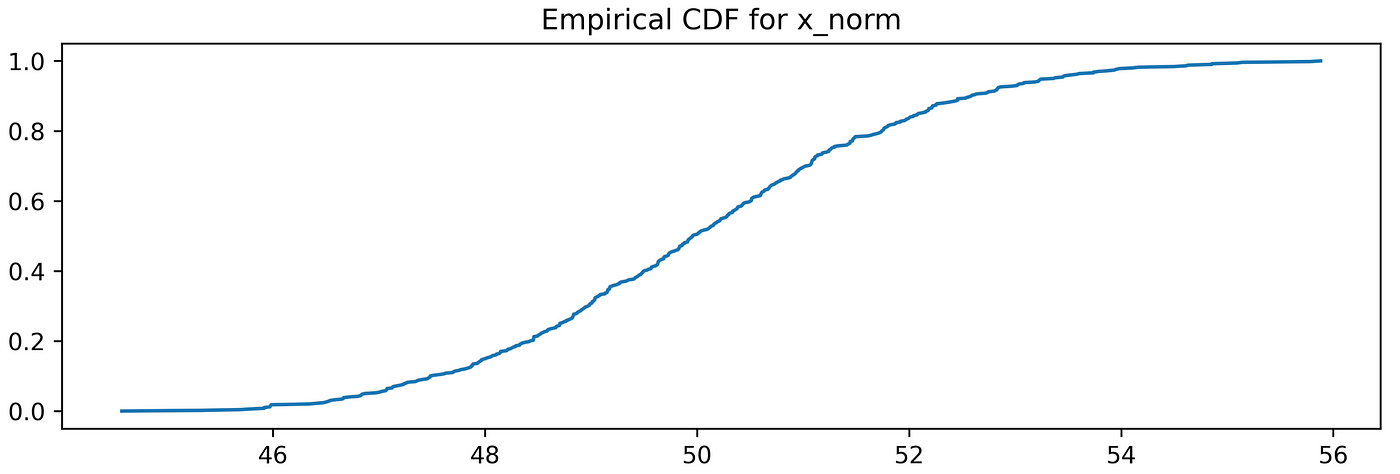
Just by observing those representations is it possible to formulate some ideas about the theoretical models that better fit our data. It is also possible to calculate the empirical distribution function:plt.plot(np.sort(x_norm), np.linspace(0, 1, len(x_norm)))plt.title(‘Empirical CDF for x_norm’)
Another graphical instrument that can come in help is the QQ plot, which shows on the y-axis the quantiles of the observed data VS the theoretical quantiles of the mathematical model.
With the term quantile, we identify the portion of observations that are below a specific value, the quantile. For example, the 0.75 quantile (or 75%) is the point where 75% of the data (sample) is below this value and 25 % is above.from scipy import statsstats.probplot(x_norm, plot=plt)
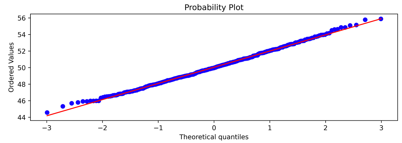
When points on the plot tend to lay on the diagonal line, it means that the data(the sample) are fitting the Gaussian model in a “good” way.
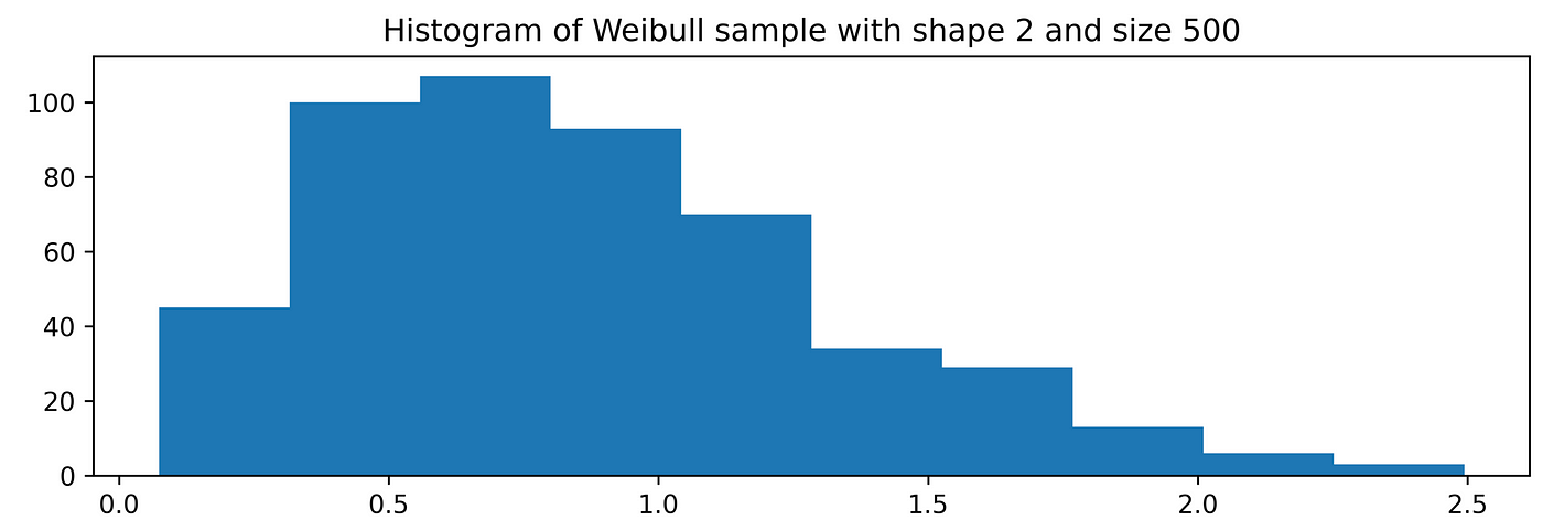
If we have another kind of observations, for example, a Weibull density function we can do the following:x_wei = np.random.weibull(2, 500) # A Weibull sample of shape 2and size 500plt.hist(x_wei)
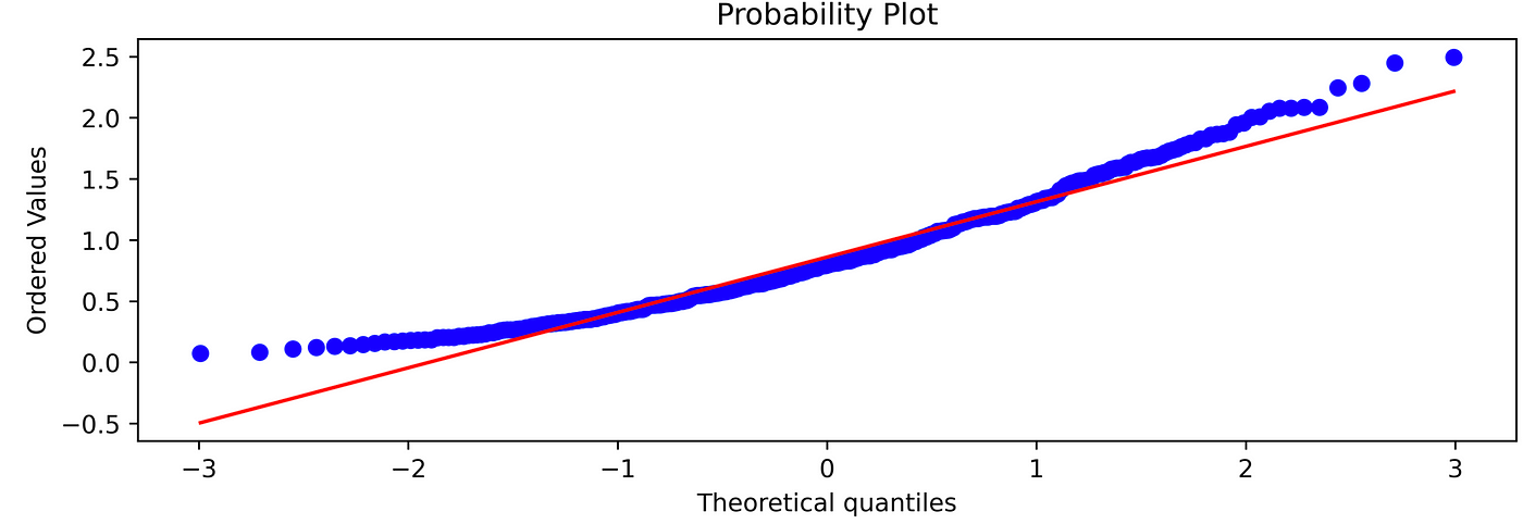
And the relative QQ plot:stats.probplot(x_wei, plot=plt)
Mills form
Edit description
relentless-creator-2481.ck.page
Choosing the right function
We saw that in some circumstances the type of model (function) can be deducted from by the structure and the nature of the model. Then a model is chosen and we verify if it follows the observed data.
In other cases the graphical representation may come in help: form the shape of the histogram it is possible to approximate the function that better represents the data, however, this method can be subject to bias.
A method absent from bias, for choosing the right function that fits data the best, is the Pearson criterion.
The Pearson criterion derives from the resolution of a differential equation that “generates” a family of different types of function that represents different empirical distributions. That function depends exclusively on four different characteristics:
- mean
- variance
- asymmetry
- kurtosis
When standardizing the distribution, the type of curve (function) only depends on the measure of asymmetry and kurtosis.
Parameter estimation
Once the function that better represents the data is chosen, it is necessary to estimate the parameters that characterize this model based on the available data. Some of the most common methods include a method of moments estimators, least squares, and maximum likelihood estimators. In this introduction we will dig into the following methods:
- the naive method
- the method of moments
- maximum-likelihood
The naive method is the most basic one and it is quite intuitive: it consists in estimating the parameters of the model by estimating, for example, the average of a sample drawn from a normal distribution with the mean of the sample under study>>> print(np.mean(x_norm))
50.03732572479421
The method of moments
The method of moments consists of expressing the population moments as functions of the parameters of interest. It is then set equal to the theoretical moments determined by the chosen function and the number of parameters to estimate.
Let’s have a look at how to tackle this issue with python:x_gamma = np.random.gamma(3.5, 0.5, 200) # simulate a gamma distribution of shape 3.5 and scale (λ) 0.5mean_x_gamma = np.mean(x_gamma) # mean of the datavar_x_gamma = np.var(x_gamma) # variance of the datal_est = mean_x_gamma / var_x_gamma # lambda estimation (rate)a_est = (mean_x_gamma ** 2) / l_est # alpha estimationprint(‘Lambda estimation: {}’.format(l_est))print(‘Alpha estimation: {}’.format(a_est))Lambda estimation: 2.25095711229392
Alpha estimation: 1.2160321117648123
The maximum likelihood method
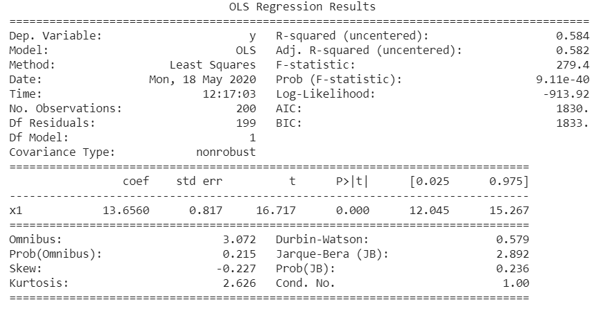
The maximum likelihood method is a method used in inferential statistics. It starts by having the density function 𝑓(𝑥,θ). It consists of estimating θ by maximizing its likelihood function or, in practice, it is often convenient to work with the natural logarithm of the likelihood function, called the log-likelihood.
Let’s see it in action:# generate datax = np.linspace(0,20, len(x_gamma))y = 3*x + x_gammaimport statsmodels.api as smols = sm.OLS(y, x_gamma).fit()print(ols.summary())
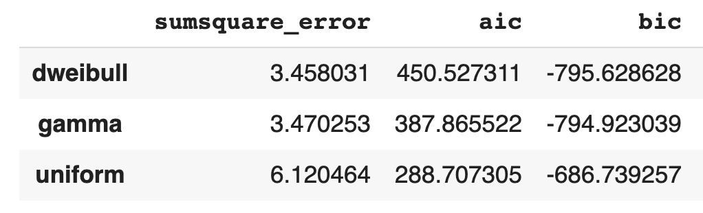
A very useful package is the fitter package, which by default estimates the distribution from which the sample is drawn. It is quite useful since it is not needed to know the likelihood function, but it is enough to only specify the sample and a list of distributions to test can be passed:#!pip install fitterfrom fitter import Fitterf = Fitter(x_gamma, distributions=[‘gamma’, ‘dweibull’, ‘uniform’])f.fit()f.summary()
Assessment of the goodness of a predictor
The assessment of the goodness of a predictor (cost function, loss function) is needed to evaluate how good are the approximations between the observed data and the data calculated (predicted) by the model. Hence, the loss function, calculates the differences between the empiric data and the observed one, it should give the same weight to errors of the same magnitude but a different sign and should increase when errors increase. Loss functions can be relative or absolute. Between the most common loss functions we can have:
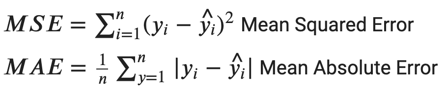
Where 𝑦 are the observed values and 𝑦̂ the theoretical (predicted) values. Often, those values are multiplied by 100 in order to express the value in percentage terms.
Let’s look at an example from a sample drawn from a Poisson distribution:import pandas as pddef dpois(x,mu):“””Calculates the density/point estimate of the Poisson distribution“””from scipy.stats import poissonresult=poisson.pmf(k=x,mu=mu)return resultx_poi = np.random.poisson(2.5, 200)lambda_est = np.mean(x_poi)table_os = pd.Series(x_poi).value_counts().sort_index().reset_index().reset_index(drop=True)table_os = table_os.valuesfreq_os = []freq_ex = []for i in range(len(table_os)):freq_os.append(table_os[i][1])freq_ex.append(dpois(x = range(0, np.max(x_poi) + 1), mu=lambda_est) * 200)from sklearn.metrics import mean_absolute_erroracc = mean_absolute_error(freq_os, freq_ex[0])print(‘Mean absolute error is: {:.2f}’.format(acc))acc_prc = acc / np.mean(freq_os) * 100print(‘Mean absolute percentage error is: {:.2f}’.format(acc_prc))Mean absolute error is: 3.30
Mean absolute percentage error is: 14.84
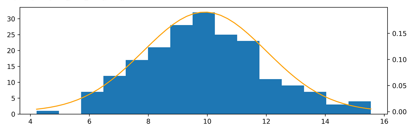
Another example of assessing the goodness of a predictor can be done by overlapping the density function with the data:x_norm = np.random.normal(10, 2, 200)(n, bins, patches) = plt.hist(x_norm, bins=15)table_os = pd.Series(x_norm).value_counts().sort_index().reset_index().reset_index(drop=True)table_os = table_os.valuesdef dnorm(x, mean=0, sd =1):“””Calculates the density of the Normal distribution“””from scipy.stats import normresult=norm.pdf(x,loc=mean,scale=sd)return resultx_fit = np.linspace(start=np.min(x_norm), stop=np.max(x_norm))y_fit = dnorm(x_fit, mean=np.mean(x_norm), sd = np.std(x_norm))fig, ax = plt.subplots(1, 1)ax.hist(x_norm, bins=15)ax2 = ax.twinx()ax2.plot(x_fit, y_fit, c=’orange’)plt.draw()
Statistical tests
It is possible to do a different statistical test to assess the goodness of fit, meaning how good the theoretical model fits the data. Those tests take into account the sample under a “global” point view, taking into account all the characteristics of the sample under study (mean, variance, the shape of the distribution…) and are distribution-agnostic, meaning they are independent of the distribution under study.
The first test under analysis, to assess the goodness of fit is the χ2 (chi-square). It is based on the comparison between the empirical frequencies (expected frequencies) and the observed frequencies, built on the desired density function. The χ2 can be used both for discrete and continuous variable and its mathematical formula is the following:
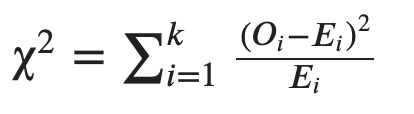
Where 𝑂𝑖 are the observed frequencies, 𝐸𝑖 the theoretical frequencies and 𝑘 the number of classes or intervals. This statistic is asymptotically distributed around a random variable denominated χ2 with 𝑘−𝑝−1 degree of freedom, where 𝑝 is the number of parameters estimated by the model.
The null hypothesis is rejected when the statistical value falls below a certain threshold, hence when the p-value is higher than the pre-fixed significance level.
The test is valid under the following conditions:
- the sample should be big enough (since the distribution is asymptotic χ2)
- The number of expected frequencies for each class cannot be less than 5.
- It is needed to apply the Yates correction for continuity (continuity correction), which consists in subtracting 0.5 from the difference between each observed value and its expected value |𝑂𝑖−𝐸𝑖|.
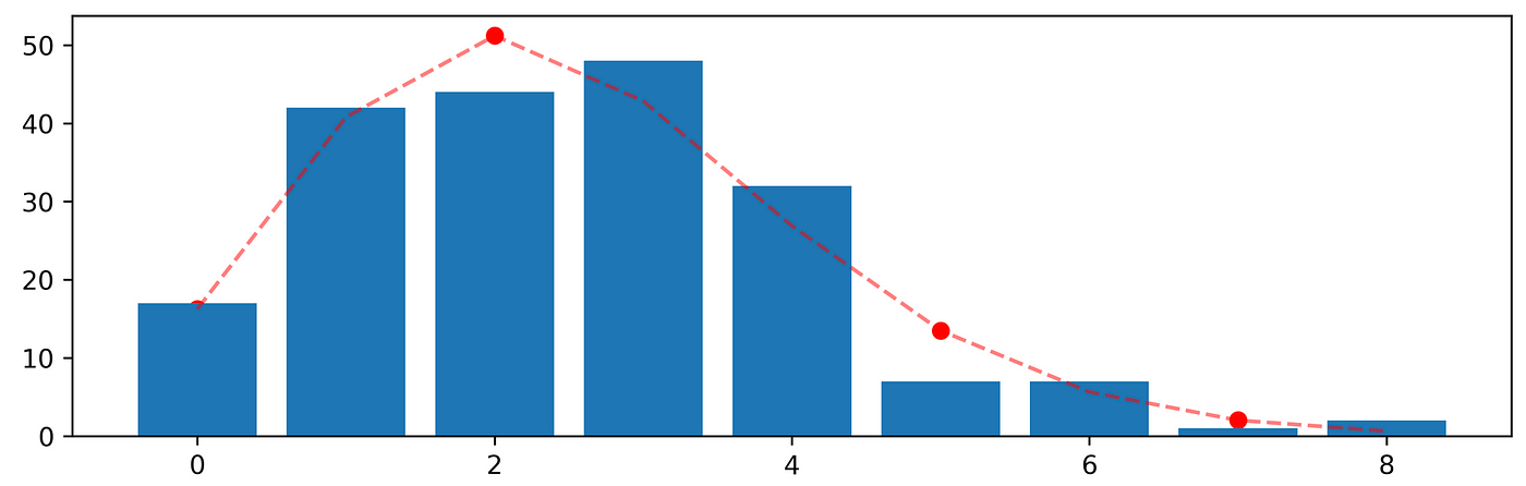
Let’s see how to implement it:import scipyobs = np.bincount(x_poi)lam = x_poi.mean()expected = scipy.stats.poisson.pmf(np.arange(len(obs)), lam) * len(x_poi)chi2 = scipy.stats.chisquare(obs, expected)[1]print(‘Chi-sqaure significance level is: {:.4f}’.format(chi2))Chi-sqaure significance level is: 0.4288
plt.bar(list(range(0, len(obs))), height=obs)plt.scatter(list(range(0, len(expected))), expected,c=’red’)plt.plot(expected,c=’red’, alpha=.5, linestyle=’dashed’)
In case of a continuous variable, in this case coming from a gamma distribution, with parameters estimated from the observed data, it can be possible to proceed as follows:a = 3.5 # shape parametermean, var, skew, kurt = gamma.stats(a, moments=’mvsk’)x = np.linspace(gamma.ppf(0.01, a), gamma.ppf(0.99, a), 1000) # percent point function# Generate random numbers from the gamma distribution with paramter shape of 3.5r = gamma.rvs(a, size=1000)plt.plot(x, gamma.pdf(x, a), lw=5, alpha=0.6)plt.hist(r, density=True, alpha=0.2)
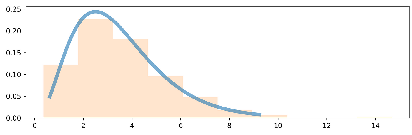
# Compute the chi-sqaure test between the random sample r and the observed frequencies xfrom scipy.stats import chisquarechisquare(r, x)>>> Power_divergenceResult(statistic=2727.3564204592853, pvalue=3.758371304737685e-160)
The null hypothesis for the chi-square test is that there is no relation between the observed and expected frequencies, however, in this case, the p-value is less than the significance level of 0.05, thus we reject the null hypothesis.
Another widely used statistical test is the Kolmogorov-Smirnov Goodness of fit test. This test is a non-parametric test that can be used both for discrete data, continuous data binned in classes (However, some authors do not agree on this), and continuous variables. This test is based on the comparison of the distance between the empirical distribution function of the data and the cumulative distribution function of the related distribution.
The Kolmogorov-Smirnov test is more powerful than the chi-square test when the sample size is not too great. For large size samples, both the tests have similar power. The most serious limitation of the Kolmogorov-Smirnov test is that the distribution must be fully specified, that is, location, scale, and shape parameters can’t be estimated from the sample. Because of those limitations, sometimes it is preferred to use the Anderson-Darling test. However, the Anderson-Darling test is available only for a small set of distributions.
In Python, we can perform this test using scipy, let’s implement it on two samples from a Poisson pdfwith parameters muof 0.6:from scipy.stats import ks_2sampfrom scipy.stats import poissonmu = 0.6 # shape parameterr = poisson.rvs(mu, size=1000)r1 = poisson.rvs(mu, size=1000)ks_2samp(r, r1)>>> Ks_2sampResult(statistic=0.037, pvalue=0.5005673707894058)
For his test, the null hypothesis states that there is no difference between the two distributions, hence they come from a common distribution. In this case, the p-value of 0.68 fails to reject the null hypothesis, in other words, the samples come from the same distribution.
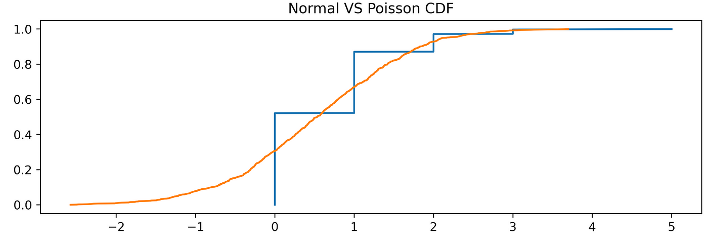
But let’s see it between a Poisson and a normal sample:from scipy.stats import normn = norm.rvs(0.6, size=1000)ks_2samp(r, n)>>> Ks_2sampResult(statistic=0.306, pvalue=9.933667429508653e-42)
On the opposite, in this case, the p-value is less than the significance level of 0.05, and it suggests that we can reject the null hypothesis, hence the two samples come from two different distributions.
We can also graphically compare the two CDF:def cdf(x, plot=True):x, y = sorted(x), np.arange(len(x)) / len(x)plt.title(‘Normal VS Poisson CDF’)return plt.plot(x, y) if plot else (x, y)cdf(r)cdf(n)
Normality Tests
Another challenge that can happen is to verify if a collected sample comes from a normal distribution, for this, there is a family of test called normality tests. One of the most powerful normality tests is the Shapiro-Wilk test, which also works very well on small samples. The normality is tested by matching two alternative variance estimates: a non-parametric estimator, calculated by a linear combination of ordered sample values, and the parametric estimator.
Scipy provides also a way to perform this test:from scipy.stats import norm, shapiron = norm.rvs(size=1000)shapiro(n)>>> (0.9977349042892456, 0.18854272365570068)
The tested null hypothesis (H0) is that the data is drawn from a normal distribution, having the p-value (0.188), in this case, we fail to reject it, stating the sample comes from a normal distribution.
Another common normality test is the Jarque-Bera test:from scipy.stats import norm, jarque_beran = norm.rvs(size=1000)jarque_bera(n)>>> (0.8127243048627657, 0.6660689052671738)
Same as before, we do not reject the null hypothesis that the data comes from a normal population.I have a newsletter 📩.Every week I’ll send you a brief findings of articles, links, tutorials, and cool things that caught my attention. If tis sounds cool to you subscribe.That means a lot for me.
Mills form
Edit description
relentless-creator-2481.ck.page
Appendix:
- Mastering Numerical Computing with NumPy: Master scientific computing and perform complex operations with ease (Umit Mert Cakmak, Mert Cuhadaroglu)
- Normality Tests in Python (https://datascienceplus.com/normality-tests-in-python/)
- Fitting a probability distribution to data with the maximum likelihood method (https://ipython-books.github.io/75-fitting-a-probability-distribution-to-data-with-the-maximum-likelihood-method/)
- FITTING DISTRIBUTIONS WITH R (https://cran.r-project.org/doc/contrib/Ricci-distributions-en.pdf)
- Distribution fitting to data (https://pythonhealthcare.org/2018/05/03/81-distribution-fitting-to-data/)